|
137 South Road Thebarton South Australia Australia 5031 |
|
| T | +61 8 8234 0511 |
| info@archimedes-consulting.com.au | |


Archimedes has contributed to a previous edition of the GEO ExPro App, ‘New Technologies’.
Automatic Curve Matching (ACM)
Fault Interpretation & Mineral Exploration
Fault interpretation and identification of clusters of magnetic sources is conducted by Archimedes using an Automatic Curve Matching (ACM) method applied to located magnetic data. ACM analyses a single magnetic anomaly along a flight line or profile extracted from a gridded Total Magnetic Intensity (TMI) field in a purely automatic manner. This method works by identifying a magnetic anomaly on a profile, comparing the unique sets of components of the observed anomaly with the one that is computed for a theoretical model, varying the parameters and accepting the solution which provides the best fit.

Profile Extraction
The first stage in the ACM method is to extract profile data and prepare for analysis. The profiles are extracted from the TMI grid in four directions: NS, EW, NW-SE and NE-SW (see Extracting Profiles). Located line data is also used where available.
Profile Analysis
Single magnetic anomalies are analysed along these profiles over the entire survey area. The profiles are then scanned to identify the anomalies in certain wave-length ranges arising from different depths. A narrow scanning window identifies high frequency anomalies, caused by shallow sources; a wide window detects deeper magnetic sources generating long wave-length anomalies (see Scanning Profiles).
Theoretical Profile Analysis
Three main theoretical models with different parameters capturing the variation in shape, size and magnetisation of potential magnetic bodies are used:
- A dyke-like body where the depth extent is much greater than the depth to the top of the body; this could used to approximate the bulk volume of the concentration of magnetized material. Dyke models are often used when searchimg for pipe-shaped magnetite breccia in mineral exploration.
- A plate or thin sheet body where the depth extent is much less than the depth to the top of the body; used to approximate sedimentary and. sometimes, volcanic horizons, and
- An edge or contact model; used to approximate geological contacts.
The observed data and profiles are extracted from grids of the TMI field and are then scanned with a range of window sizes designed to detect anomalies arising from different depths.
Observed Data and Model Data Correlation
Each single anomaly (observed and theoretical) can be represented by vertical and horizontal components, which can be further split into symmetrical and asymmetrical functions. Therefore one anomaly is represented by a unique set of four functions. The process of comparing such a set of functions representing the observed anomaly with the theoretical anomaly is known as 'curve matching'. Stringent similarity coefficient (a measure of the goodness of fit of the four matched functions) cut-offs are used to ensure best fit and high confidence results. By taking this approach a unique solution for the Magnetic Source is obtained (see Curve Matching).
Output Data
The ACM technique computes depth, magnetic susceptibility, and geometry of the causative body, as well as a similarity coefficient. This is repeated for each model and in each profile direction (see Magnetic Source Selection). The results obtained are then combined into a 3D data volume or ACM Cube (see 3D ACM Cube above right). The 3D ACM Cube is then imported into a work station where visualisation tools are used to interpret lineaments and potential faults or, in mineral exploration, to identify clusters of Magnetic Sources that could be ore bodies.
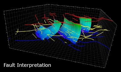
Fault Interpretation
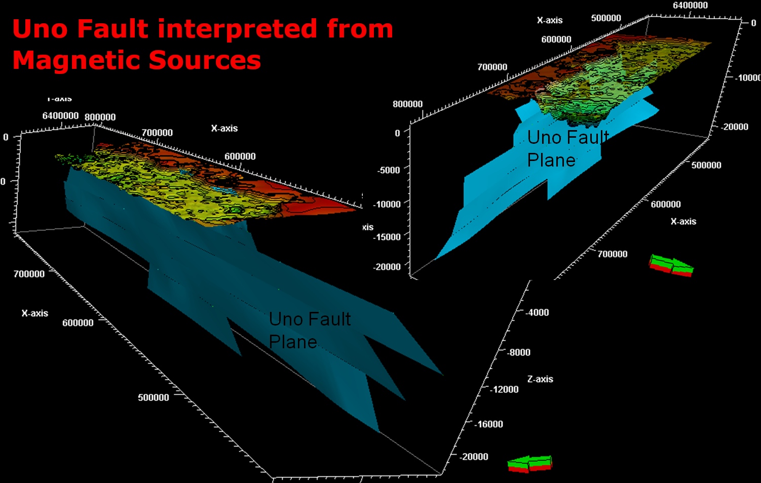
The results are further analysed to identify the most statistically significant results, which are visualized in 3D. Manual interpretation is carried out, generally in the planar view of successive depth intervals scanning through the data volume. Lineaments at multiple depths can be joined vertically, which allows identification of the large scale faults in 3D. By examining various combinations of the theoretical models, as well as different directions of the profiles and analysis of computed susceptibilities, structures within the sediments and the underlying basement are interpreted. When the ACM results from all the profile directions indicates the presence of a fault, and the lineaments can be correlated laterally and at depth, a fault plane can be gridded in 3D (see Fault Interpretation above & Uno Fault, SA).
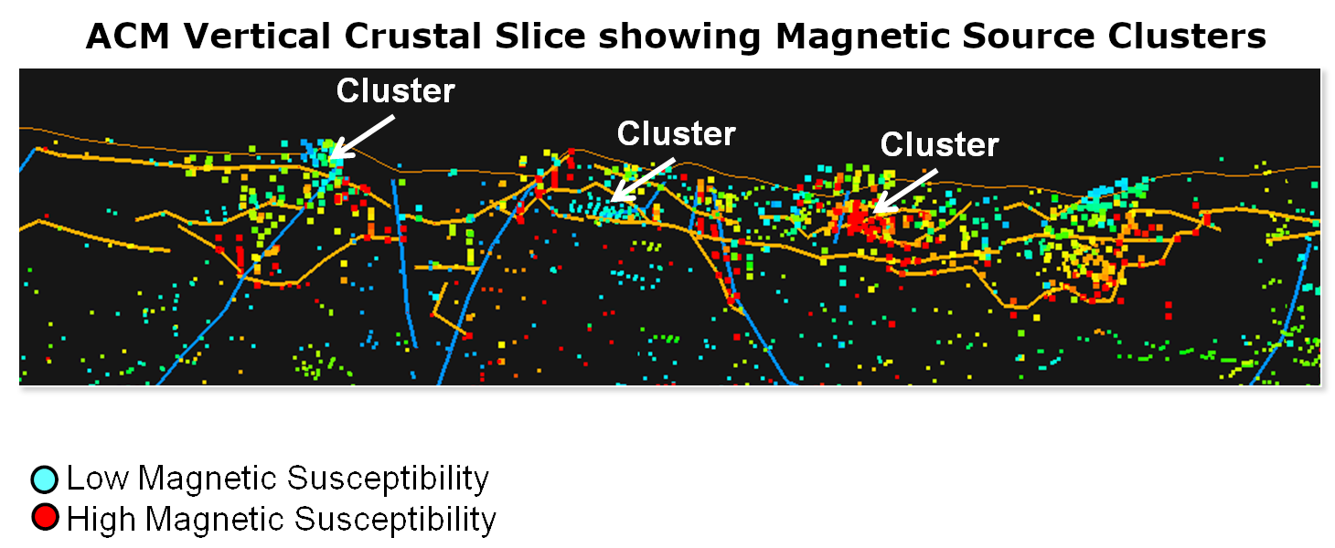
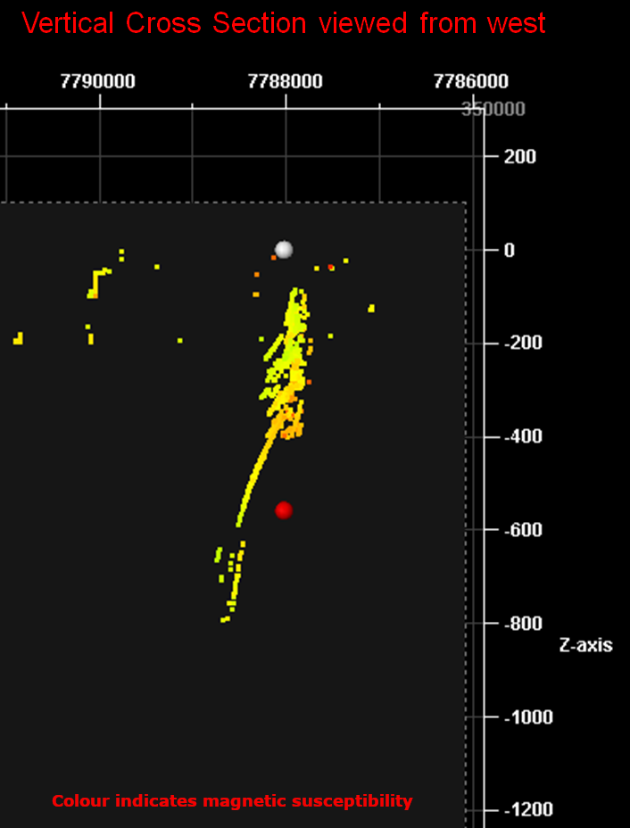
Interpretation is also conducted in vertical cross-section where a slice of a particular thickness is used to identify faults, magnetic interfaces and potential mineral exploration targets.
Mineral Exploration
ACM is applied to detect Magnetic Sources at different depths. Special input parameters and filters are designed to analyse anomalies generated by bodies located within the shallower sub-surface and deeper basement. Hundreds of thousands of Magnetic Sources detected by ACM, are interpreted in 3D using visualisation software. Each of the detected causative bodies is represented by a single point with its computed attributes. This procedure allows the rock magnetisation at different depths to be imaged and clusters of Magnetic Sources to be mapped that could represent structures typical of ore deposits. Interpretation of Magnetic Sources uses the computed magnetic susceptibility, abundance and distribution of magnetic sources as the main attributes. The magnetic susceptibilities of detected Magnetic Sources are binned into several classes which are used as key factors for the interpretation. The magnetic susceptibility data from holes drilled in the surrounding area, if available, can be used to establish the ranges of susceptibility classes to be used to map the clusters of Magnetic Sources.
Once the susceptibility range is established or inferred for the expected type of mineralisation, Magnetic Sources with lower susceptibilities can be filtered out and not displayed during the scanning of ACM-Cubes. This makes the clusters of highly Magnetic Sources more visible in 3D. The 3D ACM-Cube is sliced into Vertical Crustal Slices (VCS) (see Example of VCS); each a specific thickness depending on the type of target and continuously scanned using a small increment which allows zones and clusters of high susceptibility Magnetic Sources to be detected, and their 3D geometry be captured. Once potential targets are identified (Possible Target), Petrel's visualisation tools are used to zoom into and rotate the target to determine if it meets the criteria for a potential ore body (see ACM Cluster Video). ACM technology has also been used to create 3D voxel models of volcanic layers based on the magnetic susceptibilities computed by ACM. The magnetic field generated by the voxel models can be subtracted from the total magnetic intensity field producing a sub-volcanic magnetic field that can then be analysed and interpreted using Horizon Mapping and Fault Detection.
Summary
Archimedes approach to the interpretation of high resolution aeromagnetic data allows the detection in 3D of faults, associated structures and even fracture patterns within different sedimentary formations, as well as the underlying basement. The use of ACM in mineral exploration areas allows large areas to be quickly searched for pipe-shaped intrusive bodies, strata-hosted bodies and many other potential targets. Once these targets are located, the 3D geometry can be determined and possible drillholes designed. Results are delivered in work station ready formats for integration with other geoscience data. Our proprietary techniques extract the maximum information and deliver a detailed interpretation to aid in further exploration and development.
ACM Cluster Video